Information Security & Monty Hall Paradox

Hello, I am Kanstantsin and I am the founder of Andventum.ai. Sometimes I write tech articles about different interesting topics. Today I decided to create an article about Information Security (IS), which is quite important in FinTech

It is usually considered that AI and Data Science (DS) are quite distant from IS. In this article, I want to show this difference is not so significant.

Recently I decided to create a simple Python simulation of the Monty Hall Paradox – a brain teaser, in the form of a probability puzzle, loosely based on the American television game show Let’s Make a Deal and named after its original host, Monty Hall [I took this definition from the Wikipedia. And the next – too]. The paradox has the following definition:

Suppose you’re on a game show, and you’re given the choice of three doors: Behind one door is a car; behind the others, goats. You pick a door, say No. 1, and the host, who knows what’s behind the doors, opens another door, say No. 3, which has a goat. He then says to you, “Do you want to pick door No. 2?” Is it to your advantage to switch your choice?

The short answer is Yes, it’s my advantage to switch my choice. If I do it the winning probability is ⅔ and only ⅓ if I decide to stand on my original decision. This sounds illogical but the answer is correct. The Internet has a lot of nice and detailed explanations of why it works this way. And I don’t want to focus on the explanation.

But how does all this relate to IS? The answer is in my simulation. Please, don’t judge my code too crucially:

import random

# Returns a random door ID: 0, 1 or 2
def get_random_door():
    return random.choice([0, 1, 2])

# Set possible iterations cnts:
ITERATIONS_CNTS = [5, 10, 20, 50, 100, 200, 500, 1000, 10000, 100000]

# Results (for plots):
random_results_origin = []
random_results_changed = []

# Make experiments with all iterations:
for n_iterations in ITERATIONS_CNTS:

    # Conunters for play's reaction:
    cnt_origin_choise = 0
    cnt_changed_choise = 0

    # Do n_iterations  for experiment:
    for _ in range(n_iterations):
        # Define the door ID, which has the price:
        door_id_price = get_random_door()

        # Define the 1st choise of the player:
        door_id_player_origin = get_random_door()

        # Define a door of the host:
        doors_for_host = [item for item in [0, 1, 2] if item not in [door_id_price, door_id_player_origin]]
        door_id_host = random.choice(doors_for_host)

        # The player does not changes the mind:
        if door_id_player_origin == door_id_price:
            cnt_origin_choise += 1

        # The player changes the mind:
        door_id_player_changed = [item for item in [0, 1, 2] if item not in [door_id_host, door_id_player_origin]][0]

        if door_id_player_changed == door_id_price:
            cnt_changed_choise += 1

    # Calculate probabilities:
    prob_origin = cnt_origin_choise / n_iterations
    random_results_origin.append(prob_origin)
    
    prob_changed = cnt_changed_choise / n_iterations
    random_results_changed.append(prob_changed)

As you can see, I use the method “random” several times, because: 

• price is hidden behind a random door
• player chooses a random door
• host also needs to choose a random door in a some case

When I noticed random choice is an essential part of the algorithm I recall almost everybody, from static code analysers to university teachers, warns that “random” is an unsafe method. But everybody usually gives quite abstract explanations without practical examples. 

And I decided to replace the “random” with appropriate methods from the “secrets” lib, which is considered safer. The result is below:

import random

# Returns a random door ID: 0, 1 or 
def get_secret_door():
    return secrets.choice([0, 1, 2])

# Results (for plots):
secrets_results_origin = []
secrets_results_changed = []

# Make experiments with all iterations:
for n_iterations in ITERATIONS_CNTS:

    # Conunters for play's reaction:
    cnt_origin_choise = 0
    cnt_changed_choise = 0

    # Do n_iterations  for experiment:
    for _ in range(n_iterations):
        # Define the door ID, which has the price:
        door_id_price = get_secret_door()

        # Define the 1st choise of the player:
        door_id_player_origin = get_secret_door()

        # Define a door of the host:
        doors_for_host = [item for item in [0, 1, 2] if item not in [door_id_price, door_id_player_origin]]
        door_id_host = secrets.choice(doors_for_host)

        # The player does not changes the mind:
        if door_id_player_origin == door_id_price:
            cnt_origin_choise += 1

# The player changes the mind:
        door_id_player_changed = [item for item in [0, 1, 2] if item not in [door_id_host, door_id_player_origin]][0]

        if door_id_player_changed == door_id_price:
            cnt_changed_choise += 1

    # Calculate probabilities:
    prob_origin = cnt_origin_choise / n_iterations
    secrets_results_origin.append(prob_origin)
    
    prob_changed = cnt_changed_choise / n_iterations
    secrets_results_changed.append(prob_changed)

Now everything is ready to run the simulation and check the results. Let’s check the result if the player will stand on the original choice. See the figure below:

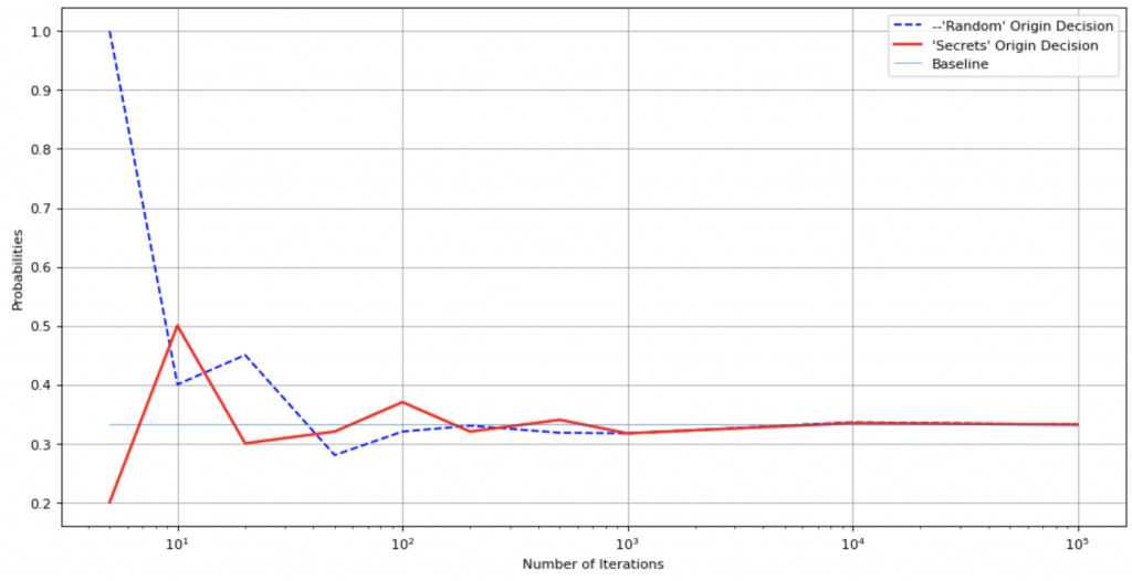
The figure has 3 charts:

• “Random” Origin Decision – success probability for the “random” method
• “Secrets” Origin Decision – success probability for the “secrets” library
• Baseline – represents the probability baseline level of ⅓ (or ⅔)

Unfortunately, we all live not in a perfect world and both “random” and “secrets” dependencies mismatch the baseline. But you can see the “random” chart doesn’t fit the baseline in a more significant way.

Next, let’s check the results for players who will decide to change their minds:

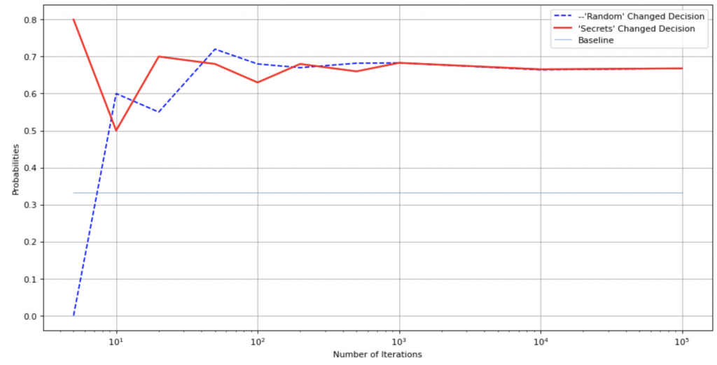
Now, let’s analyse the charts. It’s immediately noticeable that the charts get closer to the true value of the probability only with a large number of iterations – >1000. Here the Law of Large Numbers begins to work. This is correct, logical and not interesting for us.

But for a lower number of iterations, all charts have some “oscillations”. And these oscillations have significant differences between “random” and “secrets” implementations.

The “random” implementation usually has so significant mismatch that it brokes the Monty Hall Paradox for low numbers of iterations (5, 10, 20). The paradox will have the other solution: if the player stands on the original choice the success probability will strive to ½ (the opposite action will have ½ success probability too)! This solution is incorrect, but the model is correct!

The “secrets” version results will strive to correct probabilities in a much more significant number of experiments. This dependency works not in a perfect way, but works (you can create your own simulation with several iterations for each iteration from my algorithm – the Law of Large Numbers will work here too).

So, the usage of an “unsafe” method brokes our DS experiment. DS always has practical applications. The difference between ½ and ⅓ is quite big. It is about 17%! Now, you can imagine a simple example where a GameDev or gambling AI product or DS model will lose 17% more often than it was estimated. Or the required marketing campaigns budget will need 17% funds more than was forecasted. But if hackers will use this vulnerability, they can make even much more significant damage.

Note:

All the experiments were made using:

• MacBook Pro 2020 / Intel Core i5
• macOS Monterey 12.3.1
• Python 3.8.3.